Learning R for quantitative analysis

As I’ve discussed before, I learned to use the R programming language (using RStudio IDE) to conduct the quantitative analysis for my EdD degree. In this post, I’ll outline how I learned what I learned, and what I used that knowledge for.

All the code I wrote is viewable in the GitHub notebook found here.

How I learned

I started just using ChatGPT to help me learn the syntax to conduct the analysis I needed, but quickly realized I didn’t actually understand the code. So, I took advantage of a DataCamp subscription offer and bought a one year subscription.

I completed the Introduction to R course and Intermediate R course relatively promptly, making notes in OneNote as I went. I also used what I learned pretty much immediately to conduct the analysis I could by that point. First I completed some data cleaning and preparation, and then calculated the descriptive statistics (mostly just measures of central tendency and some other key metrics that were not mathematically difficult). Then, once I’d learned a bit more, I calculated the inferential statistics, some visualizations, and conducted a Cronbach’s alpha test for internal consistency of the data I collected.

In addition to the two courses above, I also completed the Introduction to Statistics in R course, and parts of Introduction to Regression in R and Hypothesis Testing in R to complete the work described.

Data preparation

After importing the two .csv files the data I collected was stored on, I renamed a column and combined the two sheets into one such that the analysis could take place once, and I wouldn’t have to repeat myself.

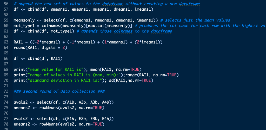
A sample of the code I wrote for calculating initial descriptive statistics

Descriptive statistics

I calculated the following descriptive statistics:

• Mean value for each motivation type (i.e. calculating the mean value of the responses for the statements within each motivation type)
• Using the largest of those mean values, I identified the motivation type each student most strongly aligned with
• Weighted mean across all motivation types to calculate the Relative Autonomy Index (RAI)
• Weighted mean like the RAI, but only using the five statements relating explicitly to the use of target grades (a measure I have named the Target Grade Affinity Index)
• The range and standard deviation for each of the measures above, though I was primarily interested in these stats for RAI and TGAI

Visualizations

I created some visualizations of these data using R (ggplot2), though I am likely to re-do these using something more ‘aesthetic’.

In order to create these visualizations, I needed to exclude the NA values since not every student participated in all three rounds of data collection. An example of this data cleaning is shown in the screenshot below:

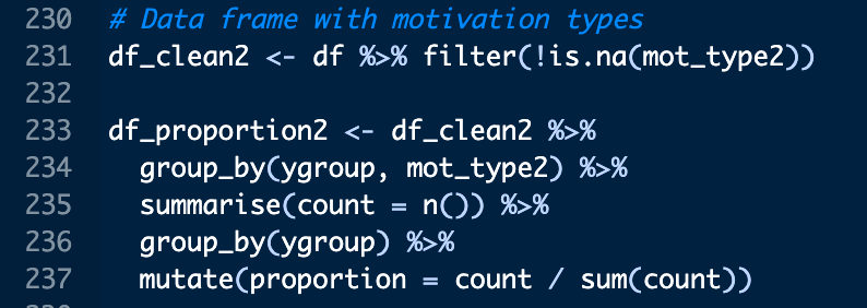
Using the dplyr package’s piping operator I was able to remove any NA values, and then group the students by year group and motivation type (in this case, for the second round of data collection), and count the number of students within each motivation type at that point. Once I did that, I calculated the proportion of students within each motivation type, since this was more easily comparable between data collection rounds.

Inferential statistics

I calculated the following inferential statistics:

• Spearman Rank Correlation Coefficient between RAI and TGAI to identify the extent to which these may be related (I know, I know, correlation does not mean causation…)
• Single linear regression between RAI and TGAI, which more assuredly confirmed there was a relationship there with 99.47% confidence for Year 11 students, and 99.98% confidence for Year 10 students
• Correlation coefficient and single linear regression for the relationship between TGAI and each student’s mean target grade
• t-test for dependent means, considering the difference between the RAI values at each point in the year (i.e. each data collection point)
• Stuart-Maxwell test to identify the change in motivation type through the year
• Cronbach’s alpha for internal consistency; this required me to negatively code the ‘controlled’ motivation types (since a high positive response from an ‘autonomous’ motivation type should necessitate an equally high negative response from a ‘controlled’ motivation type)

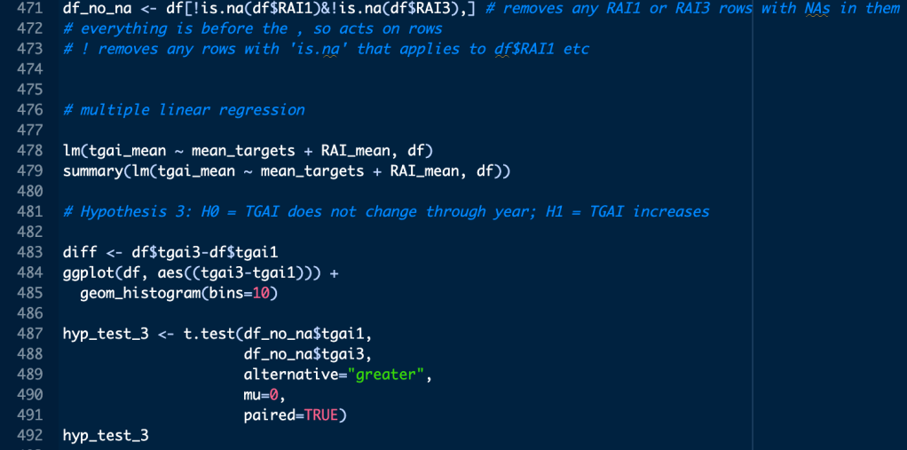
This screenshot shows a sample of the inferential statistics code. Just like with the other parts of the code, where appropriate I added comments throughout so I could go back to the code and know what I did, even though I haven’t completed any projects in R since!

While I would certainly not suggest I am an expert at R and I still have lots to learn, I am much more comfortable with it than I was when I started, and once I’ve brushed up on my Python a bit more, I might come back to this too…

Again, all the code I wrote is viewable in the GitHub notebook found here.